
Freezing a row or column in Excel is a great way to improve not only the design of your spreadsheet but its functionality as well. Frozen (also referred to as locked) rows, columns, or individual cells stay on your screen even while you’re scrolling, allowing you to create headers and key data entries.
Make finding important data or comparisons easier by taking advantage of this feature on Excel for Mac. This article goes in-depth about all aspects of freezing a row, column, or cell to make your life easier when working with the leading spreadsheet application for Mac systems.
Freeze rows and columns in Excel for Mac
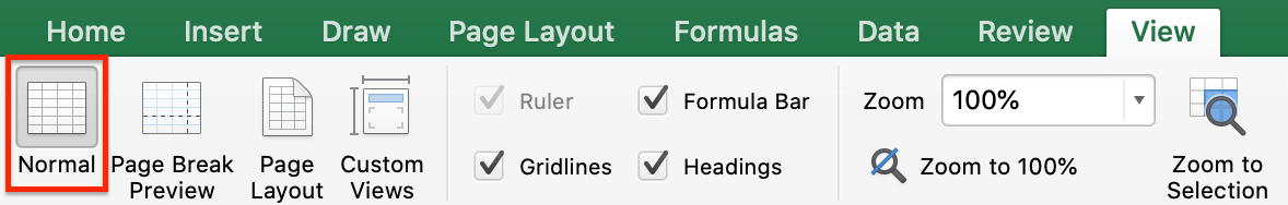
Before you can start freezing and locking, you need to ensure that you’re in the right view mode. After opening Excel and the document you’re working on, switch to the View tab in your Ribbon interface, and make sure that the Normal view is selected.
After completing this, you can proceed with the appropriate steps described below.
Freeze the top row
- Open the document you want to work on in Excel.
- Switch to the View tab in your Ribbon interface, located on top of the Excel window.
-
Click on the Freeze Top Row icon. This will automatically freeze and lock the very first row in your document. (1)
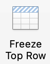
- The freeze is indicated by the bottom line of the row becoming darker than other lines, showing that the row is currently frozen.
Freeze the first column
- Open the document you want to work on in Excel.
- Switch to the View tab in your Ribbon interface, located on top of the Excel window.
-
Click on the Freeze First Column icon. This will automatically freeze and lock the very first column in your document. (A)
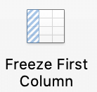
- The freeze is indicated by the right-side line of the column becoming darker than other lines, showing that the column is currently frozen.
Freeze the top row and the first column
-
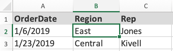
Open the document you want to work on in Excel, then select the B2 cell.
- Switch to the View tab in your Ribbon interface, located on top of the Excel window.
-
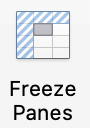
Click on the Freeze Panes icon. This will automatically freeze and lock the very first row and column in your document. (A and 1)
- The freeze is indicated by the bottom-line of the row and the right-side line of the column becoming darker than other lines, showing that they’re currently frozen.
Freeze as many rows or columns as you want
If you wish to freeze multiple columns and/or rows, you can do it as long as the top row and column of your document is included.
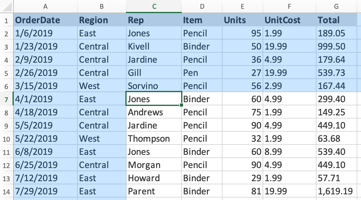
For example, selecting the C7 cell will freeze the rows and columns highlighted with blue.
All you have to do is select the column to the right of the last column you want frozen, select the row below the last row you want frozen, and click Freeze Panes.
How to unfreeze rows or columns
To unfreeze rows and columns, go to the View tab in your Ribbon and click on the Unfreeze Panes button. This will remove the frozen marks from your rows and columns, allowing you to return your document to normal in an instant.
Are you interested in other Microsoft Office guides and tutorials? Make sure to check out our dedicated Help Center section to find all the information you need about the leading office suite in the entire world. No questions are left unanswered.